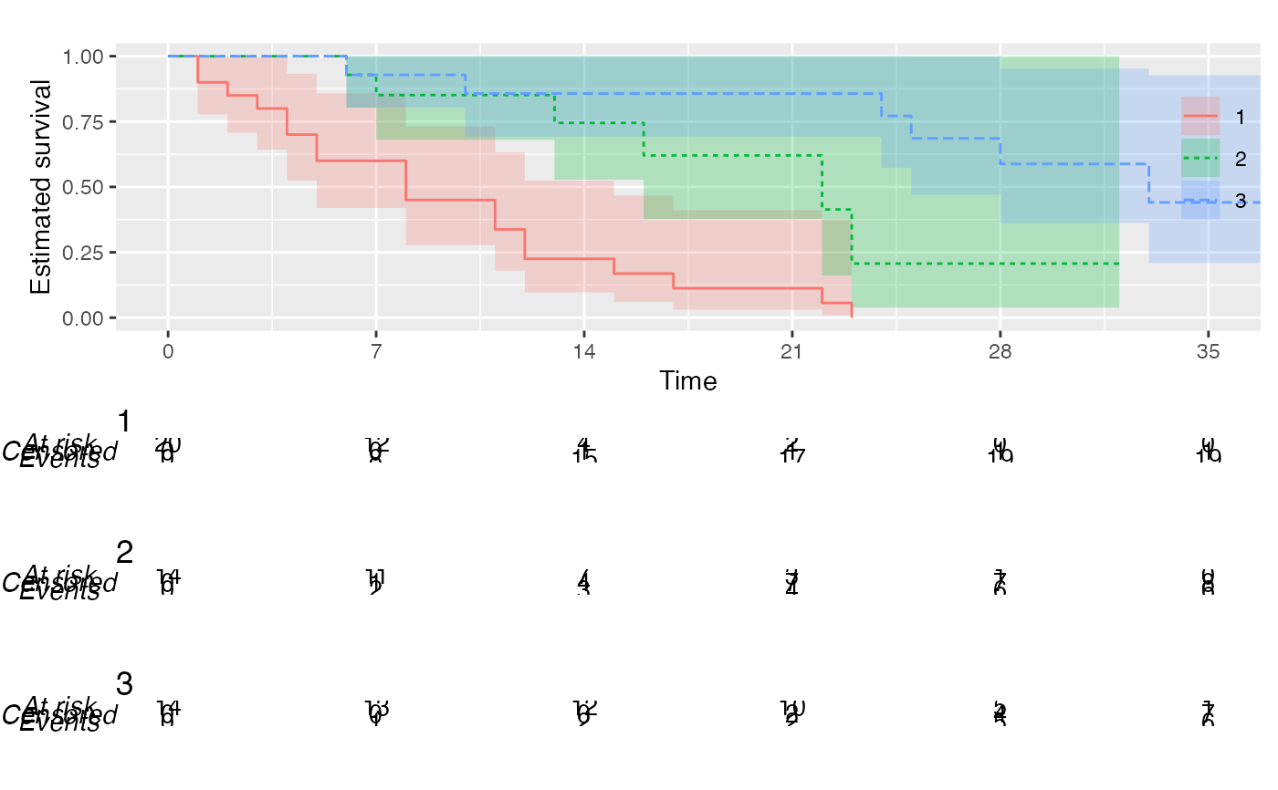
Produce Kaplan–Meier plots in the style recommended following the KMunicate study by TP Morris et al. (doi:10.1136/bmjopen-2019-030215 ).
Usage
KMunicate(
  fit,
  time_scale,
  .risk_table = "KMunicate",
  .reverse = FALSE,
  .theme = NULL,
  .color_scale = NULL,
  .fill_scale = NULL,
  .linetype_scale = NULL,
  .annotate = NULL,
  .xlab = "Time",
  .ylab = ifelse(.reverse, "Estimated (1 - survival)", "Estimated survival"),
  .title = NULL,
  .alpha = 0.25,
  .rel_heights = NULL,
  .ff = NULL,
  .risk_table_base_size = 11,
  .size = NULL,
  .legend_position = c(1, 1)
)
Arguments
- fit
A
survfitobject.- time_scale
The time scale that will be used for the x-axis and for the summary tables.
- .risk_table
This arguments define the type of risk table that is produced.
- .reverse
If
reverse = TRUE, then the plot uses 1 - survival probability on the y-axis. Defaults toKMunicate, where the cumulative number of events and censored are calculated. Another possibility issurvfit, which will use the default numbers returned bysummary.survfit(e.g. number of events and censored per interval)..risk_tablecan also beNULL, in which case the risk table will be omitted from the plot.- .theme
ggplottheme used by the plot. Defaults toNULL, where the defaultggplottheme will be used.- .color_scale
Colour scale used for the plot. Has to be a
scale_colour_*component, and defaults toNULLwhere the default colour scale will be used.- .fill_scale
Fill scale used for the plot. Has to be a
scale_fill_*component, and defaults toNULLwhere the default fill scale will be used.- .linetype_scale
Linetype scale used for the plot. Has to be a
scale_linetype_*component, and defaults toNULLwhere the default linetype scale will be used.- .annotate
Optional annotation to be added to the plot, e.g. using
ggplot2::annotate(). Defaults toNULL, where no extra annotation is added.- .xlab
Label for the horizontal axis, defaults to Time.
- .ylab
Label for the vertical axis, defaults to Estimated survival if
.reverse = FALSE, to Estimated (1 - survival) otherwise.- .title
A title to be added on top of the plot. Defaults to
NULL, where no title will be included.- .alpha
Transparency of the point-wise confidence intervals
- .rel_heights
Override default relative heights of plots and tables. Must be a numeric vector of length equal 1 + 1 per each arm in the Kaplan-Meier plot. See
cowplot::plot_grid()for more details on how to use this argument.- .ff
A string used to define a base font for the plot.
- .risk_table_base_size
Base font size for the risk table, given in pts. Defaults to 11.
- .size
Thickness of each Kaplan-Meier curve. Defaults to
NULL, whereggplot2's default will be used.- .legend_position
Position of the legend in the plot. Defaults to
c(1, 1), which corresponds to top-right of the plot. It is also possible to pass a string, as inggplot2, e.g."none"to suppress the legend. N.B.: Legend justification is modified accordingly. Seeggplot2::theme()for more details on how to place the legend of the plot.