autoplot method for multisimsum objects — autoplot.multisimsum • rsimsum

autoplot can produce a series of plot to summarise results of simulation studies. See vignette("C-plotting", package = "rsimsum") for further details.

Usage

# S3 method for multisimsum
autoplot(
  object,
  par,
  type = "forest",
  stats = "nsim",
  target = NULL,
  fitted = TRUE,
  scales = "fixed",
  top = TRUE,
  density.legend = TRUE,
  zoom = 1,
  zip_ci_colours = "yellow",
  ...
)

Arguments

object: An object of class multisimsum.
par: The parameter results to plot.
type: The type of the plot to be produced. Possible choices are: forest, lolly, zip, est, se, est_ba, se_ba, est_density, se_density, est_hex, se_hex, est_ridge, se_ridge, heat, nlp, with forest being the default.
stats: Summary statistic to plot, defaults to bias. See summary.simsum() for further details on supported summary statistics.
target: Target of summary statistic, e.g. 0 for bias. Defaults to NULL, in which case target will be inferred.
fitted: Superimpose a fitted regression line, useful when type = (est, se, est_ba, se_ba, est_density, se_density, est_hex, se_hex). Defaults to TRUE.
scales: Should scales be fixed (fixed, the default), free (free), or free in one dimension (free_x, free_y)?
top: Should the legend for a nested loop plot be on the top side of the plot? Defaults to TRUE.
density.legend: Should the legend for density and hexbin plots be included? Defaults to TRUE.
zoom: A numeric value between 0 and 1 signalling that a zip plot should zoom on the top x% of the plot (to ease interpretation). Defaults to 1, where the whole zip plot is displayed.
zip_ci_colours: A string with (1) a hex code to use for plotting coverage probability and its Monte Carlo confidence intervals (the default, with value zip_ci_colours = "yellow"), (2) a string vector of two hex codes denoting optimal coverage (first element) and over/under coverage (second element) or (3) a vector of three hex codes denoting optimal coverage (first), undercoverage (second), and overcoverage (third).
...: Not used.

Value

A ggplot object.

Examples

data("frailty", package = "rsimsum")
ms <- multisimsum(
  data = frailty,
  par = "par", true = c(trt = -0.50, fv = 0.75),
  estvarname = "b", se = "se", methodvar = "model",
  by = "fv_dist", x = TRUE
)
#> 'ref' method was not specified, Cox, Gamma set as the reference

library(ggplot2)
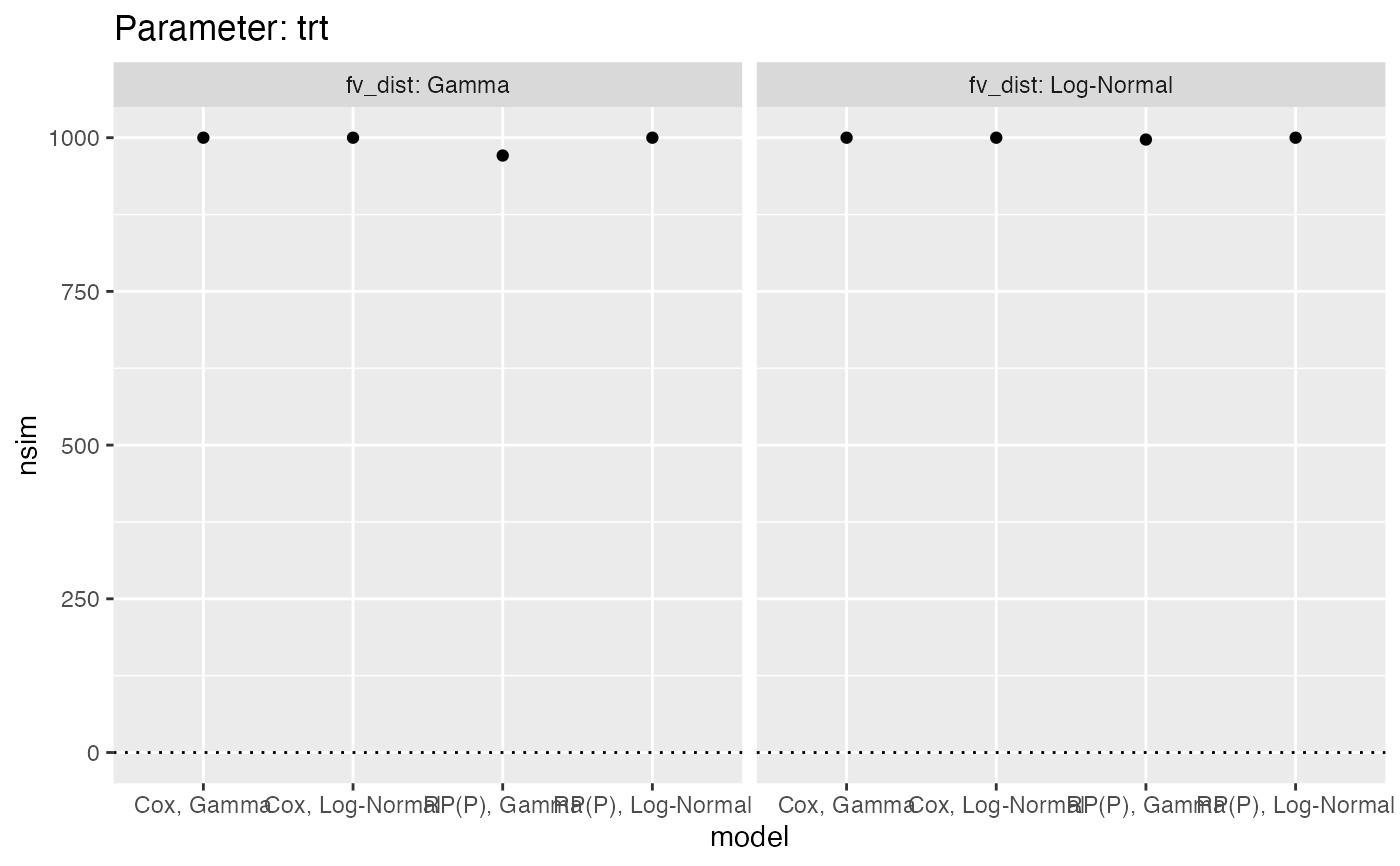
autoplot(ms, par = "trt")

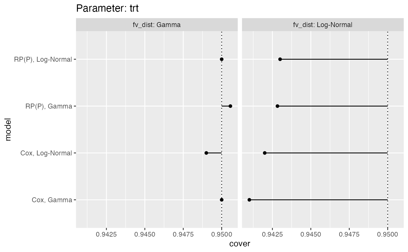
autoplot(ms, par = "trt", type = "lolly", stats = "cover")

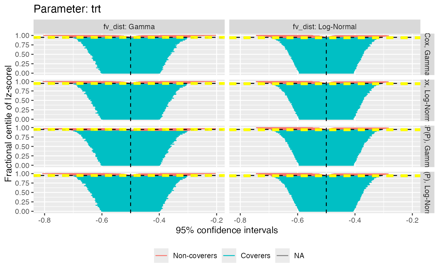
autoplot(ms, par = "trt", type = "zip")
#> Warning: Removed 32 rows containing missing values or values outside the scale range
#> (`geom_segment()`).

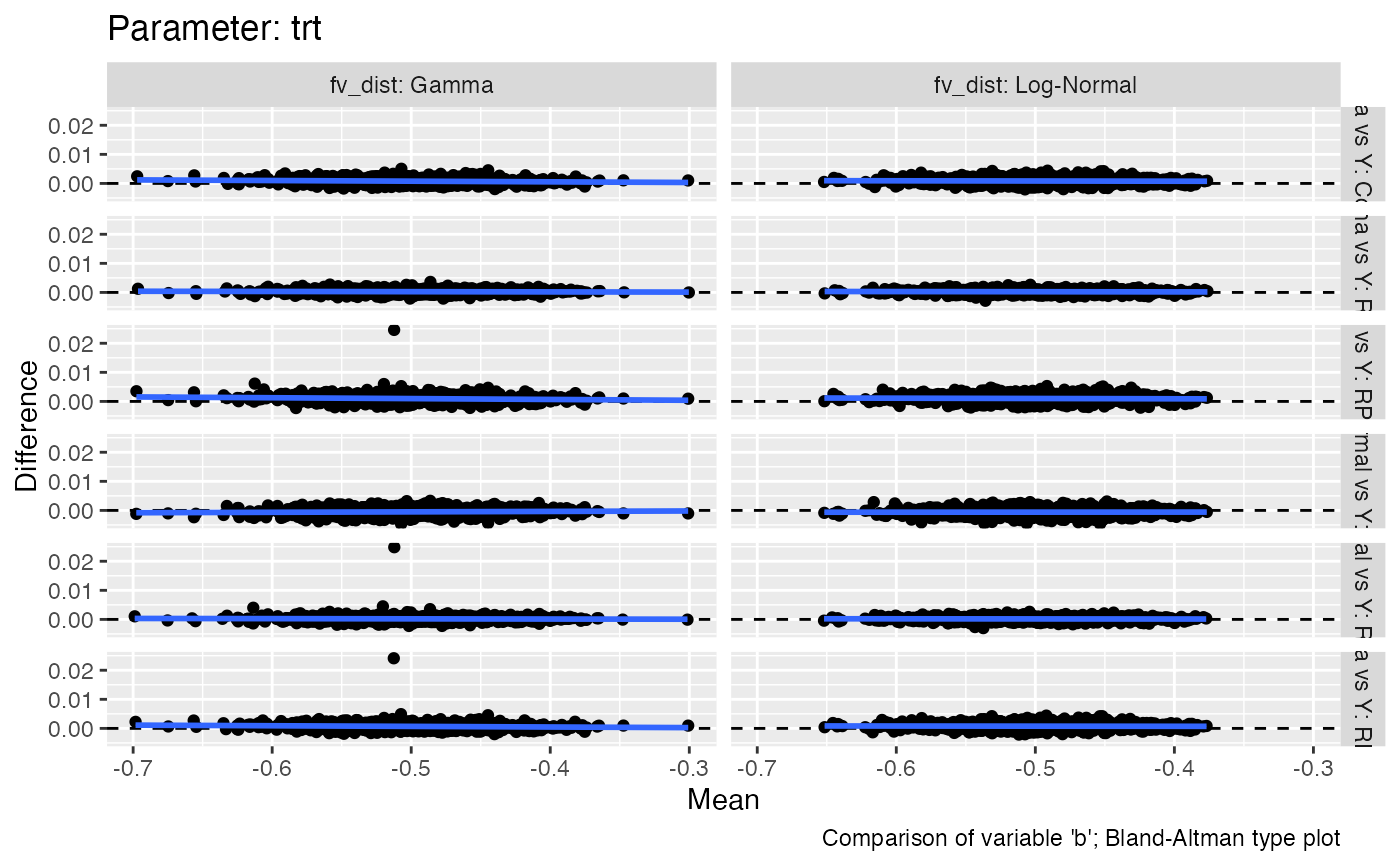
autoplot(ms, par = "trt", type = "est_ba")
#> `geom_smooth()` using formula = 'y ~ x'
#> Warning: Removed 96 rows containing non-finite outside the scale range
#> (`stat_smooth()`).
#> Warning: Removed 96 rows containing missing values or values outside the scale range
#> (`geom_point()`).